4 The Whole Game: Hello `ggplot2`

4.1 Why This Week Matters

This week gives you the whole course workflow in a small form. You will open a project, run R code, make a plot, and push your work to GitHub.

flowchart LR
  A[Raw data] --> B[Inspect]
  B --> C[Clean]
  C --> D[Summarize]
  D --> E[Plot]
  E --> F[Report]
  F --> G[Share]

You are not expected to understand every detail yet. The goal is to see the full path once so future weeks feel less mysterious. Later chapters will slow down and explain each part.

The most important habit this week is to work in small steps. Run a little code, check what happened, then make the next change.

4.2 Learning Goals

By the end of this week, you should be able to:

open the weekly project in Positron (or RStudio as fallback)
run a few lines of R code
create a basic ggplot2 scatterplot
run a complete R script and inspect its plot
commit and push your work to GitHub
describe what the plot shows in plain language

4.3 Vocabulary

Term	Meaning in this course	Example
project	A folder that keeps the files for one piece of work together	`week_01.Rproj`
script	A file that stores R code you can run again	`week_01_follow_along.R`
Quarto document	A file that mixes text and code and can render to HTML	`week_01.qmd`
render	Build the final report or slides from a Quarto document	Render to HTML
package	Extra R tools installed outside base R	`ggplot2`, `palmerpenguins`
object	A named thing stored in R	`penguins`
function	A command that does work	`ggplot()`
argument	Information given to a function	`x = flipper_length_mm`
commit	A saved checkpoint in Git	“Add Assignment 01 plot”
push	Send local commits to GitHub	Push to origin

4.4 Before You Start

You should have access to the Assignment 01 materials and a private Assignment 01 assignment repository:

the Module 03 slide deck and Assignment 01 follow-along script
the Assignment 01 Classroom 50 link
the private repository Classroom 50 creates for you

You will use the palmerpenguins data. The data describe penguins measured near Palmer Station in Antarctica. We use this dataset because it is small, real, and friendly for a first plot.

Assignment 01 due date: Tuesday, September 15, 2026, 11:59 PM Central Time.

4.4.1 From the graph to the assignment

The graph you explored in class is the starting point for this assignment, not a separate task. After your instructor posts the Assignment 01 Classroom 50 assignment, create your private repository, clone it, and open assignment.R. Rebuild the familiar graph there: flipper length on the x-axis, body mass on the y-axis, and species mapped to color. Then add clear labels, write a short interpretation in comments, run the script, inspect the plot, commit, and push.

This sequence matters. Classroom 50 creates the private repository; it does not replace the work of cloning, editing, rendering, checking, committing, and pushing. Each step leaves evidence that the next person can review.

4.4.2 Getting your assignment repository

Use one of the two paths below. You do not need to use a terminal or the gh command-line tool for this assignment. Both paths do the same job.

Brand-new Positron user? Use its built-in Source Control to clone first.

Do not start with File → Open Folder: there is no local assignment folder yet. First copy your private repository’s Code → HTTPS address on GitHub. In Positron’s built-in Source Control, select New Folder from Git, paste that address, and choose where to save your class work. When Positron finishes cloning, open the new folder it created; then open assignment.R in the Explorer. You do not need a terminal or a separate GitHub CLI extension.

If GitHub Desktop will not open

Do not keep clicking or try random fixes. Your work is safe in your private GitHub repository. Use the Positron Source Control path below, or take a screenshot of the message and ask for help.

First, complete these steps no matter which path you choose:

Accept the NRES800 organization invitation in GitHub.
Open Classroom 50, sign in with that same GitHub account, and select NRES800.
Open Assignment 01 and create your private repository. Classroom 50 creates a repository for you; it is not the public course template.
Open the repository link Classroom 50 gives you. Keep this browser tab open: you will use it to verify your final push.

4.4.2.1 Path A: GitHub Desktop

Use this path if GitHub Desktop opens on your computer. On a Mac with an M1, M2, M3, or M4 chip, choose the Apple silicon download.

Open GitHub Desktop and sign in with the same GitHub account you used for Classroom 50.
Choose File → Clone repository. Select the GitHub.com tab.
Select the private Assignment 01 repository that Classroom 50 created for you. If it is not listed, return to Classroom 50 and make sure you created the repository with the same GitHub account; then reopen the clone window.
Choose a folder on your computer where you can find class work again. Click Clone. Cloning makes the first local copy of the repository.
In GitHub Desktop, choose Repository → Show in Finder/Explorer. Open that folder in Positron, then open assignment.R.

At the start of every work session, use the button in GitHub Desktop’s toolbar:

Click Fetch origin. Fetch checks GitHub for new work but does not change your files.
If the button changes to Pull origin, save and commit any work you want to keep, then click Pull origin. Pull brings the remote changes into your local copy.
If it remains Fetch origin, your local copy is already current.

When you have finished a piece of work:

Save your files in Positron and return to GitHub Desktop.
Click each changed file to review what will be saved. Leave every required file checked.
Write a short summary, such as Add labeled penguin graph, then click Commit to main. A commit is a named checkpoint on your computer.
Click Push origin. Push copies the commit from your computer to GitHub.
Refresh the repository page you kept open in your browser. You should see the new commit message and your updated files.

4.4.2.2 Path B: Positron’s built-in Source Control (clone first, then open the folder)

Use this path if Git is installed on your computer. It is equally correct, and it is the path to use if GitHub Desktop will not open. If you do not see Source Control in Positron, take a screenshot and ask for help before making changes.

In your private Assignment 01 repository on GitHub, click Code, select the HTTPS tab, and copy the repository address.
In Positron, choose New Folder from Git from the Welcome screen. If you already have a folder open, open the Command Palette and search for Workspaces: New Folder from Git.
Paste the repository address, choose a parent folder for your class work, and select Create Folder. When Positron asks, open the new folder and trust it only because it is your NRES800 assignment repository.
Open assignment.R. The Source Control icon in Positron’s left Activity Bar is where you will see changes, commits, and remote actions.

At the start of every work session:

Select the Source Control icon.
Select … (More Actions) → Fetch. Fetch checks GitHub for new commits without changing your files.
If Positron shows incoming commits or a down arrow, select … → Pull. Pull brings those commits into your local files. Save or commit your own work first if you have changes you want to keep.

When you have finished a piece of work:

Save your files. In Source Control, click a changed file to review the before-and-after view.
Click the + beside each file you want in the checkpoint. The files move to Staged Changes.
Type a short commit message, such as Add labeled penguin graph, and click Commit. This saves the checkpoint locally.
Select … → Push. If Positron asks you to sign in to GitHub, sign in with the account that owns your Classroom 50 repository.
Refresh the repository page in your browser and confirm the commit message and changed files appear there.

What the words mean: clone = make the first local copy; fetch = check/download remote history without changing files; pull = bring remote changes into local files; commit = save a named local checkpoint; push = send local commits to GitHub. Do not use Discard Changes unless you intend to throw away that file’s uncommitted work.

4.5 The Main Idea

Data analysis is a workflow, not a single command.

In this course, a good workflow means:

You know where your files are.
You can run the code again.
You can see the output.
You can explain what the output means.
You can share the work through GitHub.

The first plot is a way to practice the workflow. The plot matters, but the repeatable process matters more.

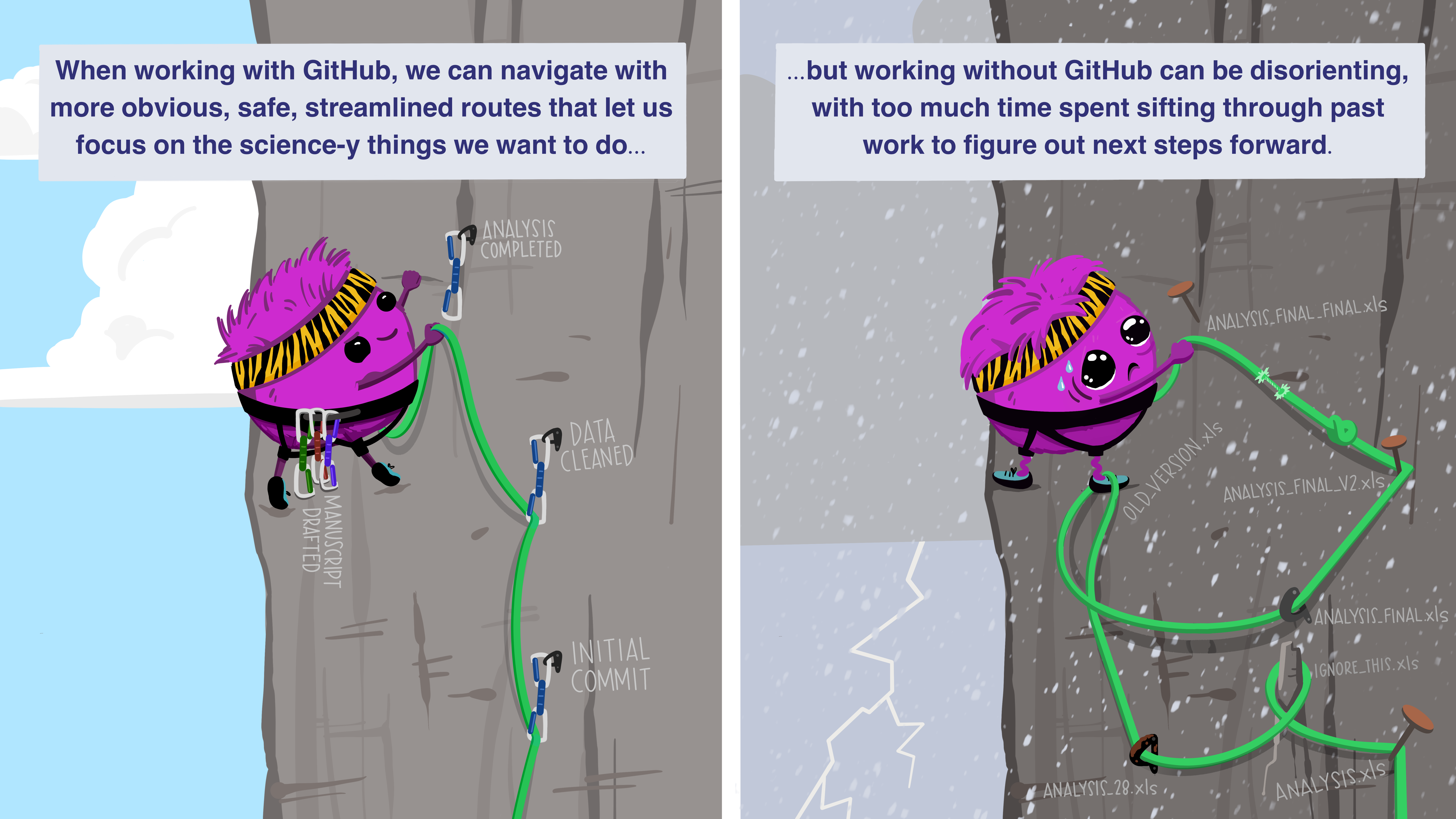
Figure 4.1: Two-panel illustration comparing a researcher using GitHub to follow a clear route through a climbing landscape, with labeled checkpoints for an initial commit, a cleaned dataset, and completed analysis, to a researcher without GitHub tangled in multiple poorly named analysis files in a snowstorm.

Illustration by Allison Horst, licensed CC BY 4.0. The illustration is used here unchanged.

4.6 Build The Workflow

4.6.1 Load Packages

R packages add functions and data that are not available in base R. Assignment 01 uses palmerpenguins and ggplot2.

library(palmerpenguins)
library(ggplot2)

Read this code as:

load the palmerpenguins package
load the ggplot2 package
make their data and functions available in this R session

If R says a package is missing, the package needs to be installed before it can be loaded.

4.6.2 Inspect The Data

Before you plot data, look at it.

penguins

This prints the penguins data. You are not trying to memorize every row; you are learning to notice the column names and the kind of information stored in them.

Useful questions:

How many rows are there?
What are the column names?
Which columns are numbers?
Which columns are categories?
Are there missing values?

4.6.3 Count Groups

Counting groups is a simple way to check what is in the data.

count(penguins, species)

This asks: how many rows belong to each penguin species?

You can also count two variables together:

count(penguins, species, island)

This asks: how many rows are there for each combination of species and island?

4.6.4 Make A Scatterplot

A scatterplot shows the relationship between two numeric variables.

ggplot(
  data = penguins,
  mapping = aes(
    x = flipper_length_mm,
    y = body_mass_g
  )
) +
  geom_point()

This plot puts flipper length on the x-axis and body mass on the y-axis. Each point is one penguin.

4.6.5 Add Color

Color can show groups.

ggplot(
  data = penguins,
  mapping = aes(
    x = flipper_length_mm,
    y = body_mass_g,
    color = species
  )
) +
  geom_point()

Now each point is colored by species. This makes it easier to see whether species differ in flipper length and body mass.

4.6.6 Add Labels

Labels make a plot easier for another person to read.

ggplot(
  data = penguins,
  mapping = aes(
    x = flipper_length_mm,
    y = body_mass_g,
    color = species
  )
) +
  geom_point() +
  labs(
    title = "Penguin body mass and flipper length",
    x = "Flipper length (mm)",
    y = "Body mass (g)",
    color = "Species"
  )

The code did not change the data. It changed how the result is communicated.

4.7 Read The Code

This code has several nested parts:

ggplot(
  data = penguins,
  mapping = aes(
    x = flipper_length_mm,
    y = body_mass_g,
    color = species
  )
) +
  geom_point()

Read it slowly:

ggplot() starts a plot.
data = penguins says which data frame to use.
mapping = aes(...) says how variables in the data connect to visual parts of the plot.
x = flipper_length_mm puts flipper length on the horizontal axis.
y = body_mass_g puts body mass on the vertical axis.
color = species colors points by species.
geom_point() draws points.
The + adds another layer to the plot.

The most common beginner mistake is to forget that ggplot2 uses + to add plot layers. The + must come at the end of the line that is being continued.

4.8 Check Your Work

After you run the code, check these things:

Does a plot appear?
Is flipper length on the x-axis?
Is body mass on the y-axis?
Are the points colored by species?
Does the plot have a title and clear axis labels?
Can you say one sentence about what the plot shows?

A good first interpretation might be:

Penguins with longer flippers tend to have higher body mass, and the species form different clusters.

This sentence does not claim too much. It describes what is visible in the plot.

4.9 Common Problems

Symptom	Likely cause	First thing to try
`could not find function "ggplot"`	`ggplot2` is not loaded	Run `library(ggplot2)`
`object 'penguins' not found`	`palmerpenguins` is not loaded	Run `library(palmerpenguins)`
R prints `+` in the console and waits	A command is incomplete	Press `Esc`, then check parentheses and `+` signs
The plot appears but has no color	`color = species` is missing or outside `aes()`	Put `color = species` inside `aes()`
The R script does not run	Code works line-by-line but not as a script	Make sure the script loads all needed packages
Work is not on GitHub	Commit or push step was skipped	Check the Git pane and push your commit

4.10 Try It

Base task:

Make the scatterplot with flipper length on the x-axis, body mass on the y-axis, and color by species. Add a title and clear labels.

Extension:

Change the plot so color shows island instead of species. Then write one sentence comparing the two plots. Which color choice helps you understand the data better?

4.11 Connect To The Assignment

Assignment 01 turns the graph from class into a reproducible script. It is not only about making the correct plot. It is about proving that you can complete the whole workflow:

Open Assignment 01 in Classroom 50 and create your private repository.
Clone the repository with GitHub Desktop or Positron and open assignment.R.
Rebuild the flipper-length/body-mass graph, with species mapped to color.
Add readable labels and write a two-sentence interpretation of a visible pattern.
Run assignment.R and inspect the plot.
Complete the README, commit your changes, and push to GitHub.

If the plot works on your computer but the rendered file or GitHub version is missing, the workflow is not finished.

4.12 Finish The Professional Workflow

Before you submit or commit, look at the final output instead of only checking whether the code ran. Your script should leave behind one visible result that another person can understand: a printed summary, a plot, or a saved file. Add a one-sentence note in your workflow document that says what the result shows and where it came from.

Before you stop, complete this checklist:

Run the complete R script.
Check that the plot appears without an error.
Save your files.
Commit with a short message, such as Add Assignment 01 penguin plot.
Push to GitHub.
Confirm that GitHub shows your latest work.

This finish step is part of data science. A result that only exists on one computer is fragile. A rendered, committed, and pushed result is easier to review, revise, and trust.