flowchart LR
  A[Cleaned, checked table] --> B["ggplot(data, aes())"]
  B --> C[Geom by data type]
  C --> D[Facets, scales, labels, palette]
  D --> E[Caption states the pattern]
11 Visualizing Wrangled Data
11.1 Why This Week Matters
A figure is a summary you look at. Every choice in it (which rows, which column goes on which axis, what the colors mean, whether panels share a scale) is a decision, the same way every summarize() was. A figure built from the raw file inherits every trap in the raw file. A figure built from a table you cleaned and checked does not.
We practise on two Great Lakes Fishery Commission tables you already know, via TidyTuesday 2021-06-08: commercial catch (fishing.csv, Module 05, thousands of pounds, 1867-2015) and fish stocking events (stocked.csv, Module 04, number of fish, 1950-2018). The question: lake trout collapsed around 1950 and managers started stocking. Did catch come back?
Your project draft (due Sun Nov 29) needs at least three figures. This chapter is the reference for them, and its last part shows how to join two tables if your project needs one.
11.2 Learning Goals
By the end of this module, you should be able to:
- build a plot from its three parts: data, aesthetics, geom
- tell an aesthetic (mapped from a column) from a setting (one fixed value)
- choose a geom by data type
- use facets, a log scale, labels with units, and a colorblind-safe palette
- join two tables by a key, and audit the join with row counts and
anti_join() - add a figure with
fig-capandfig-altto a Quarto report
11.3 Vocabulary
| Term | Meaning |
|---|---|
| Aesthetic | A visual property (x, y, color, fill, size) mapped from a column, inside aes(). Gets a legend |
| Setting | A visual property with one fixed value for everything, outside aes() (color = "steelblue") |
| Geom | The shape that draws the data: geom_line(), geom_col(), geom_histogram(), geom_boxplot(), geom_point() |
| Facet | One small panel per group: facet_wrap(~ lake), or a grid with facet_grid(rows ~ cols) |
| Scale | How data values become positions or colors: scale_x_log10(), scale_color_viridis_d() |
| Key | The column(s) that identify which rows match in a join (lake and year) |
left_join() |
Keep every row of the left table; add matching columns from the right (NA when there is no match) |
anti_join() |
Rows of the left table with no match in the right. The join audit |
11.4 The Main Idea
Every ggplot has the same three parts:
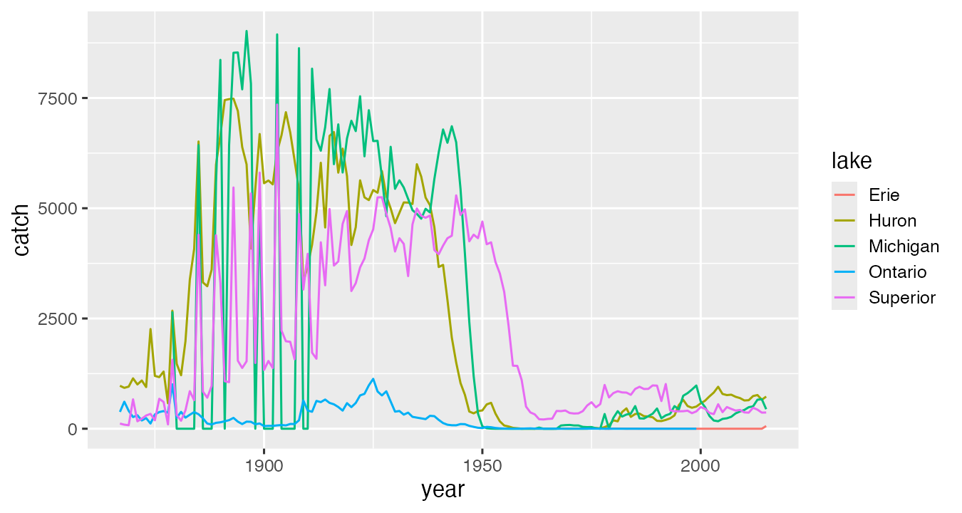
ggplot(trout, aes(x = year, y = catch, color = lake)) +   # data + aesthetics
  geom_line()                                             # geom
Layers are added with +, not |>. Here trout is a table we built and checked first: whole-lake lake trout catch per lake and year (U.S. total rows plus Canada total rows, the Module 05 trap), 606 rows.
11.5 Build The Workflow
11.5.1 Aesthetic or setting
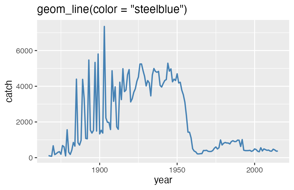
Inside aes(), a value is mapped from a column and gets a legend. Outside aes(), it is one fixed value for everything. The classic bug is a fixed value inside aes():
ggplot(superior, aes(x = year, y = catch, color = "steelblue")) + geom_line()ggplot treats "steelblue" as a column whose every value is the word “steelblue”, picks the first default color (salmon pink), and adds a legend that says “steelblue”. The fix is geom_line(color = "steelblue").
aes().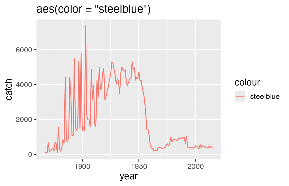
aes().11.5.2 Pick the geom by the data
| Your data | Geom | Example |
|---|---|---|
| A number over time | geom_line() |
Catch by year |
| One number per category | geom_col() |
Total catch by lake, 2000-2015 |
| Distribution of one number | geom_histogram(), geom_boxplot() |
Fish per stocking event |
| Two numbers | geom_point() |
Fish stocked vs catch |
geom_col() plots a number your table already has. geom_bar() counts rows for you (it is count() inside ggplot).
A missing bar is not a zero bar. In the 2000-2015 lake trout totals, Lake Ontario has no bar at all because its catch rows end in 1999. A caption should say so.
11.5.3 Scales: when everything piles up
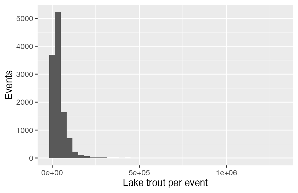
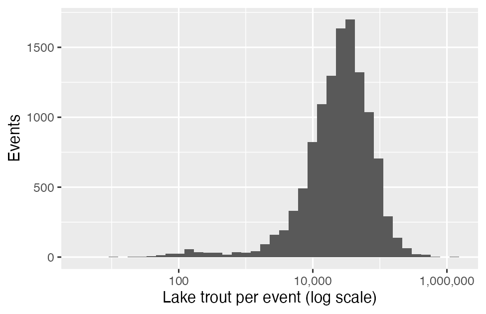
Lake trout per stocking event has a median of 27,167 fish and a maximum of 1,300,000. On a regular axis nearly every event lands in the first bar. scale_x_log10() spreads them out. A log scale cannot show 0, so filter zeros first (one event here) and say so in the caption.
11.5.4 Facets
ggplot(trout, aes(x = year, y = catch)) +
  geom_line() +
  facet_wrap(~ lake, scales = "free_y")
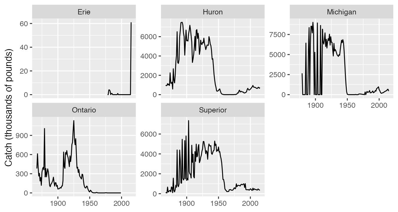
Facets replace color when there are many groups, and they do not depend on telling colors apart. scales = "free_y" gives each panel its own range, so panel heights are no longer comparable. Say that in the caption.
11.5.5 Labels with units, and color everyone can read
ggplot(trout, aes(x = year, y = catch, color = lake)) +
  geom_line() +
  scale_color_viridis_d(end = 0.85) +
  labs(
    x = NULL,
    y = "Commercial catch (thousands of pounds)",
    color = "Lake",
    title = "Lake trout catch collapsed around 1950"
  ) +
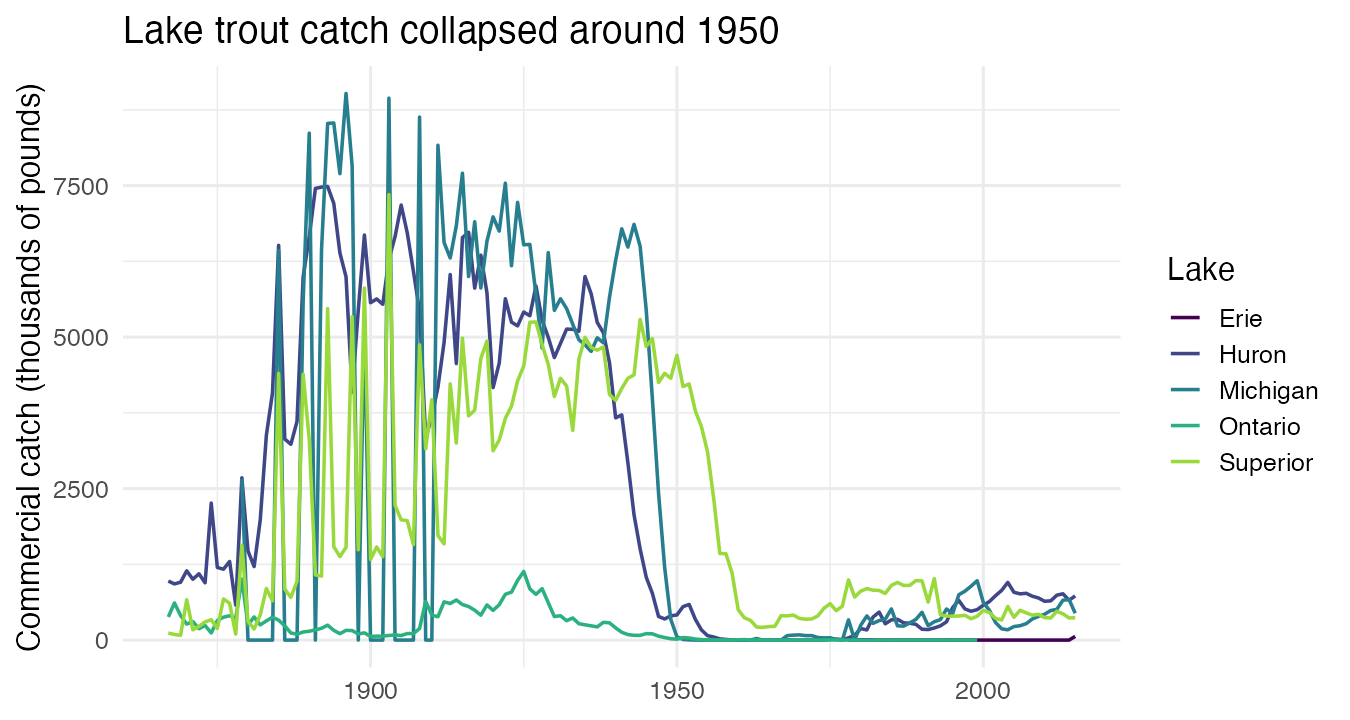
theme_minimal()- Every axis gets units. The project rubric checks this.
- A title or caption that states the finding beats one that names the variables.
viridisis built into ggplot2 and is colorblind-safe;end = 0.85drops the pale yellow that disappears on white. Color should never be the only way to read a figure: facets, line labels, or shapes back it up.
11.5.6 Joins: two tables, one key
To ask whether catch came back as stocking went up, both numbers need to be in the same row. A join matches rows of two tables by key columns.
visits |> left_join(sites, by = "site")   # every visit, plus its habitat
visits |> anti_join(sites, by = "site")   # visits whose site is not in sites
When the keys are spelled differently in the two tables (catch says "Michigan", stocking says "MI"), build a small lookup table and join it first:
lake_key <- tibble(
  lake_code = c("ER", "HU", "MI", "ON", "SU"),
  lake      = c("Erie", "Huron", "Michigan", "Ontario", "Superior")
)

stock_trout <- stocked |>
  filter(species == "LAT") |>
  group_by(lake_code = lake, year) |>
  summarize(fish_stocked = sum(no_stocked), .groups = "drop") |>
  left_join(lake_key, by = "lake_code")     # 264 rows before and after

trout_both <- trout |>
  left_join(stock_trout, by = c("lake", "year"))   # 606 rows, same as trout
Three habits make a join trustworthy:
- Count rows before and after. A lookup join should never add rows. Joining
trouttostock_troutbylakealone gives 32,877 rows and a “many-to-many relationship” warning: every catch year matched every stocking year for that lake. The key must identify one row in the table you are joining in. - Run
anti_join()both ways. 378 catch years found no stocking record, because catch records start in 1867 and lake trout stocking records start between 1950 (Michigan) and 1972 (Huron). In the other direction, 36 stocking years found no catch: 2016-2018 (catch data end in 2015), Lake Ontario after 1999, and Lake Erie before 1978. - Say what NA means. Here NA in
fish_stockedmeans “no record”, not “zero fish”. The caption should say so.
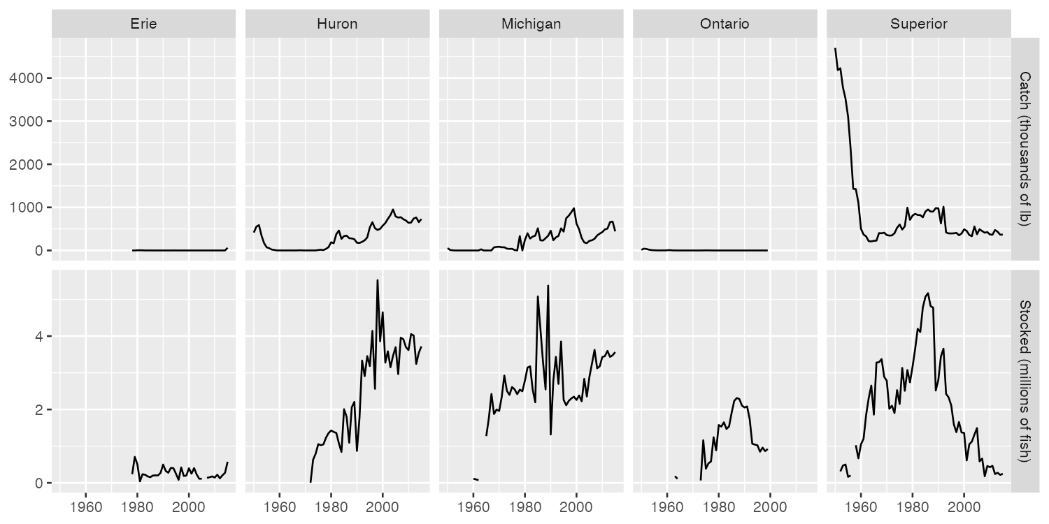
The figure uses pivot_longer() from Module 06 so catch and stocking each get a row of panels: facet_grid(measure ~ lake, scales = "free_y").
Other joins you may need for a project: inner_join() keeps only rows that match in both tables; bind_rows() stacks tables that have the same columns (for example, one file per year).
11.5.7 Figures in a Quarto report
```{r}
#| label: fig-trout
#| fig-cap: "Lake trout catch fell to near zero in Lakes Michigan and
#|   Huron by 1955 and stayed low for decades."
#| fig-alt: "Line chart of commercial lake trout catch, 1867 to 2015, one
#|   line per lake. Michigan, Huron and Superior drop sharply after 1945."
ggplot(trout, aes(x = year, y = catch, color = lake)) +
  geom_line()
```fig-capis what a reader sees: one sentence that states the pattern. The project rubric checks for it.fig-altis what a screen reader says: what the figure shows.- The label must start with
fig-. Quarto then numbers the figure, and you can refer to it in your text as@fig-trout.
11.6 Common Problems
| You see | Why | Fix |
|---|---|---|
An error mentioning a ggplot object as data, or + ignored |
|> between ggplot layers |
Layers join with + |
object 'year' not found in ggplot() |
Columns given without aes() |
ggplot(data, aes(x = year, y = catch)) |
| Line in the wrong color and a legend with one entry | A fixed value inside aes() |
Move it into the geom: geom_line(color = "steelblue") |
| Zig-zag lines jumping up and down | Several groups drawn as one line | Map the group: color = lake, or facet |
Removed n rows containing missing values |
NA values (or zeros on a log scale) | Not an error. Decide whether to filter, and say so in the caption |
| Rows multiply after a join, many-to-many warning | Key is too short (by = "lake", not c("lake", "year")) |
Join by every column that identifies a row; check nrow() |
| All NA in the joined columns | Keys spelled differently (MI vs Michigan) |
Lookup table first; check with anti_join() |
11.7 Try It
In your Module 05 repo, class/week_08_follow_along.R: Sections 1-3 with Challenges 1 and 2, then Section 4 (joins) and Section 5 (one figure in your project report).
11.7.1 In-Class Challenge Hints
Try each step for a few minutes before opening a hint.
TipChallenge 1, Step 1, Hint 1: the plan
Start from lake_catch, not trout (trout has only one species). Filter to whitefish, then reuse your trout ggplot() code. For the CHECK, filter to one year and sort.
TipChallenge 1, Step 1, Hint 2: closer
lake_catch |> filter(species == "Lake Whitefish") |> ggplot(aes(...)) with the same three aesthetics as the trout plot. For the CHECK: filter(species == "Lake Whitefish", year == 2015), then arrange(desc(catch)).
TipChallenge 1, Step 2, Hint 1: the plan
One lake means no color = lake. A fixed color is a setting, so where does it go?
TipChallenge 1, Step 2, Hint 2: closer
Add lake == "Michigan" to the filter, keep only x and y in aes(), and write geom_line(color = "darkgreen", linewidth = 1).
TipChallenge 2, Step 1, Hint 1: the plan
Start from stocked. Two conditions in one filter(): the species and no_stocked > 0. One box per lake means lake is x. The log goes on the axis that holds the numbers.
TipChallenge 2, Step 1, Hint 2: closer
aes(x = lake, y = no_stocked), geom_boxplot(), scale_y_log10(). For the CHECK: group_by(lake), summarize(median_event = median(no_stocked)), arrange(desc(median_event)).
TipChallenge 2, Step 2, Hint 1: the plan
Summarize first, plot second: one row per lake and year with the total in millions. The table already has the number, so which geom?
TipChallenge 2, Step 2, Hint 2: closer
group_by(lake, year), summarize(millions = sum(no_stocked) / 1e6), then ggplot(aes(x = year, y = millions)) + geom_col() + facet_wrap(~ lake).
11.8 Connect To The Assignment
Assignment 08 uses NOAA tornado records (a different dataset, the same skills): figures with units and pattern captions, and a join. It opens Wed Nov 11 and is due Sun Nov 22, 11:59 PM. The release announcement on Canvas has the link.
For your project, the draft (due Sun Nov 29) needs at least three figures with at least two geom types, captions that state the pattern, axis labels with units, and a colorblind-safe palette. If your data come in more than one table, the joins section above is the pattern: lookup table, row counts before and after, anti_join() both ways.