flowchart LR
  A["Text: split, trim, NA"] --> B["Categories: choose and order levels"]
  B --> C["Dates: pull out the part you need"]
  C --> D["Report: a table and numbers in sentences"]
12 Text, Categories, and Dates
12.1 Why This Week Matters
A file can import without a single warning and still not be ready to count. The problems hide in what the text says: two facts packed into one column, the same value spelled three ways, a placeholder like "Tree(s)" that R counts as a real name, a date column that is missing for most rows. Each of these needs one decision before you can count or plot it, and the decision belongs in your report.
This is a short module. There is no Assignment 09: the last part of class goes to your project draft (due Sun Nov 29).
12.2 Learning Goals
- Split a text column that holds two facts, trim it, and turn placeholder text into
NA(separate_wider_delim(),str_trim(),na_if()) - Make values that mean the same thing match (
str_to_lower()), and find or pull out a pattern (str_detect(),str_extract()) - Choose and order the levels of a category for a plot (
fct_lump_n(),fct_infreq(),fct_rev()), and say so in the caption - Pull out the part of a date a question needs (
year(),month(),wday()), and say which rows the dates cover - Add a
gttable and an inline value to a Quarto report
12.3 Vocabulary
| Term | Meaning |
|---|---|
| Delimiter | The text that separates two values in one string, like :: in "Acer rubrum :: Red Maple" |
| Placeholder | Text standing in for “unknown” ("Tree(s)", "::", "-"). R counts it as a value until you make it NA |
| Pattern (regular expression) | A description of text to match. "^width" means “starts with width”; "[0-9.]+" means “one or more digits or dots” |
| Level | One of the values a factor can take. Its order sets the order of bars and legend entries |
| Lumping | Combining the small levels of a factor into one "Other" level |
| Inline value | R code inside a sentence of a Quarto report, recomputed every render |
12.4 The Main Idea
The data are San Francisco’s public street tree inventory (TidyTuesday 2020-01-28): 192,987 trees, 12 columns. One row is one tree or tree site. The most common value of species is not a species:
| species | n |
|---|---|
Tree(s) :: |
11,629 |
Platanus x hispanica :: Sycamore: London Plane |
11,557 |
Metrosideros excelsa :: New Zealand Xmas Tree |
8,744 |
"Tree(s)" means the inventory did not record a species. Until you turn it into NA, every count of species, every bar chart, and every “most common tree” sentence treats it as the city’s most common tree.
12.5 Build The Workflow
12.5.1 Text: one column, two facts
species holds a scientific name and a common name joined by ::. Split on the delimiter, trim the spaces it leaves, and make empty text and the placeholder NA:
trees_sp <- trees |>
  separate_wider_delim(species, delim = "::",
                       names = c("scientific", "common"),
                       too_few = "align_start") |>
  mutate(across(c(scientific, common), str_trim),
         across(c(scientific, common), \(x) na_if(x, "")),
         scientific = na_if(scientific, "Tree(s)"))
Three details matter:
- Split on
"::", not" :: "."Tree(s) ::"has no space after the colons, so the version with spaces would not split it. too_few = "align_start"keeps rows with nothing after the::and fills the missing piece withNA, instead of stopping with an error.- After the split, 13,468 trees have no scientific name (11,629
"Tree(s)"plus 1,839"::"), and 15,086 have no common name.
12.5.2 Text: same thing, different spelling
plot_size has 525 distinct values, including "3x3" (29,166 trees) and "3X3" (12,073). Lowercasing alone brings it to 465:
trees_sp <- trees_sp |>
  mutate(
    plot_size = str_to_lower(plot_size),
    width_ft = if_else(str_detect(plot_size, "^width"),
                       as.numeric(str_extract(plot_size, "[0-9.]+")), NA)
  )
str_detect() returns TRUE or FALSE; str_extract() returns the matching text. 85,694 plots have a width; 17,017 of them say "Width 0ft". A zero-width plot is either a site with no planting strip or a placeholder: say which you assumed before you average it.
12.5.3 Categories: which levels, in what order
There are 550 common names. A bar per name is 550 bars in alphabetical order, which answers no question.
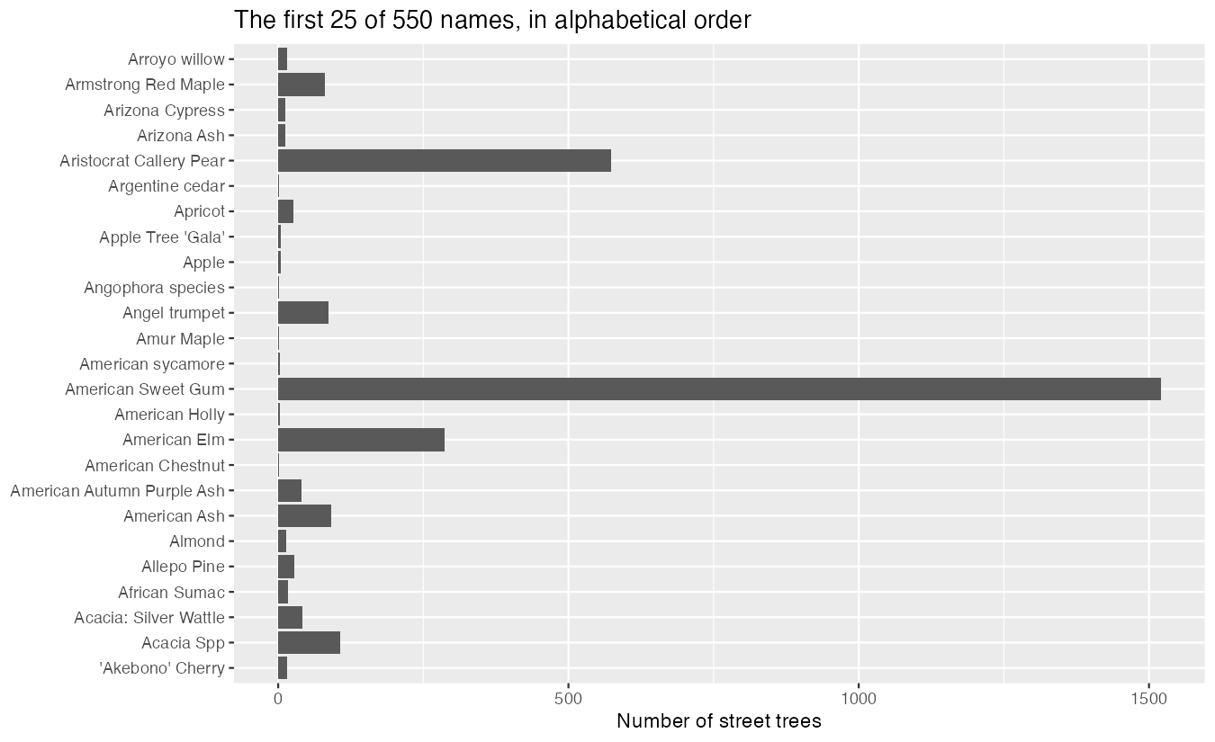
Two decisions: which levels to show, and in what order.
trees_sp |>
  filter(!is.na(common)) |>
  mutate(common = fct_lump_n(common, n = 10)) |>
  ggplot(aes(y = fct_rev(fct_infreq(common)))) +
  geom_bar()
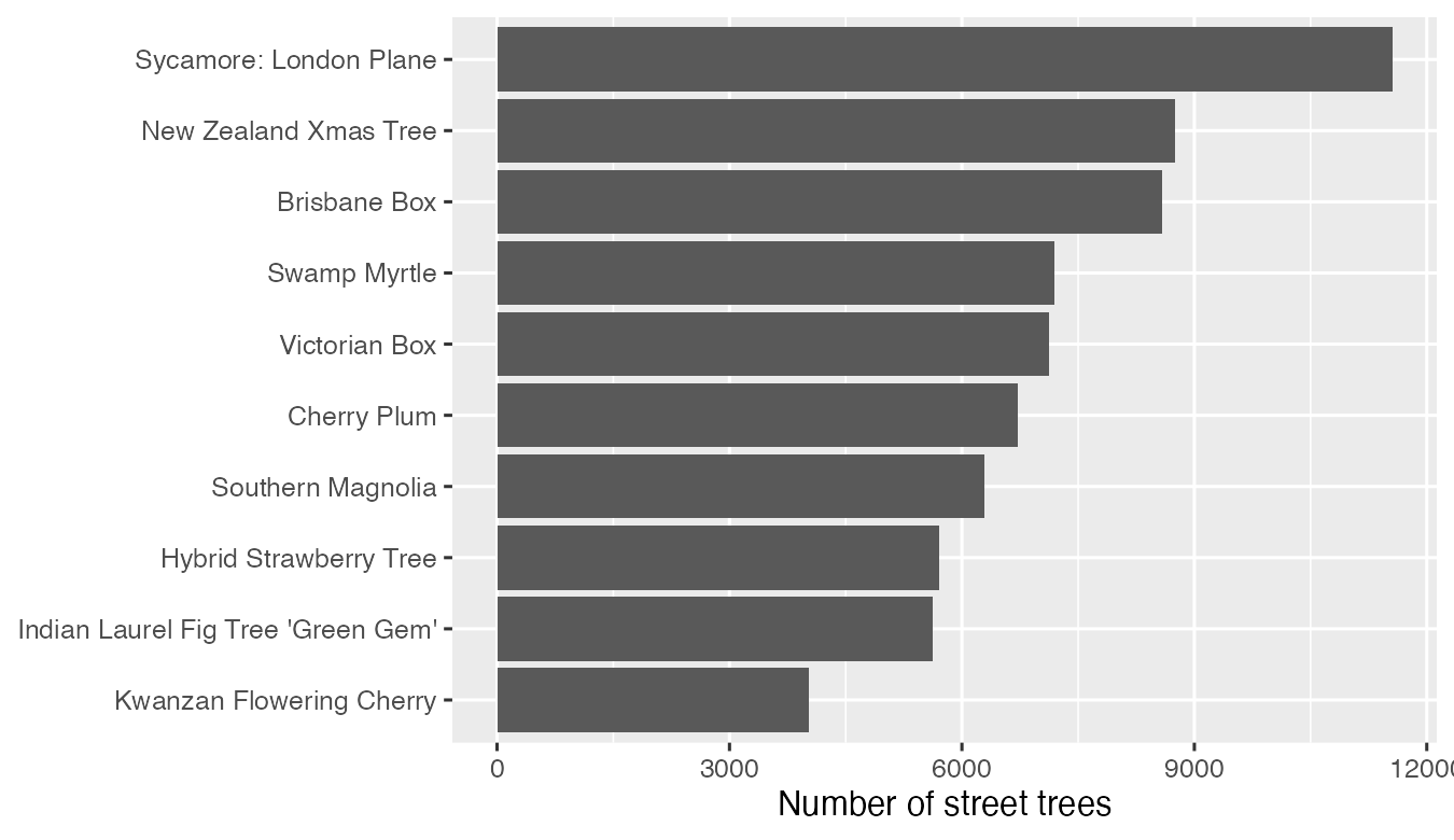
fct_lump_n() keeps the 10 most common names and puts the rest in "Other". fct_infreq() orders the levels by count, and fct_rev() flips them so the biggest bar is on top.
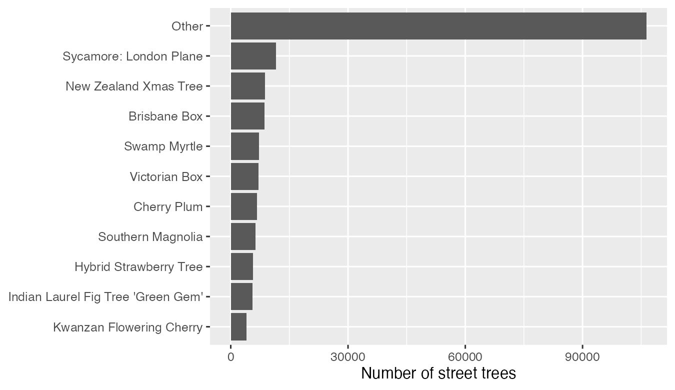
Here “Other” is 60% of named trees. Lumping is honest only if the reader is told: keep "Other" and say what it holds, or drop it with filter(common != "Other") and say the figure shows the 10 most common.
12.5.4 Dates: pull out the part you need
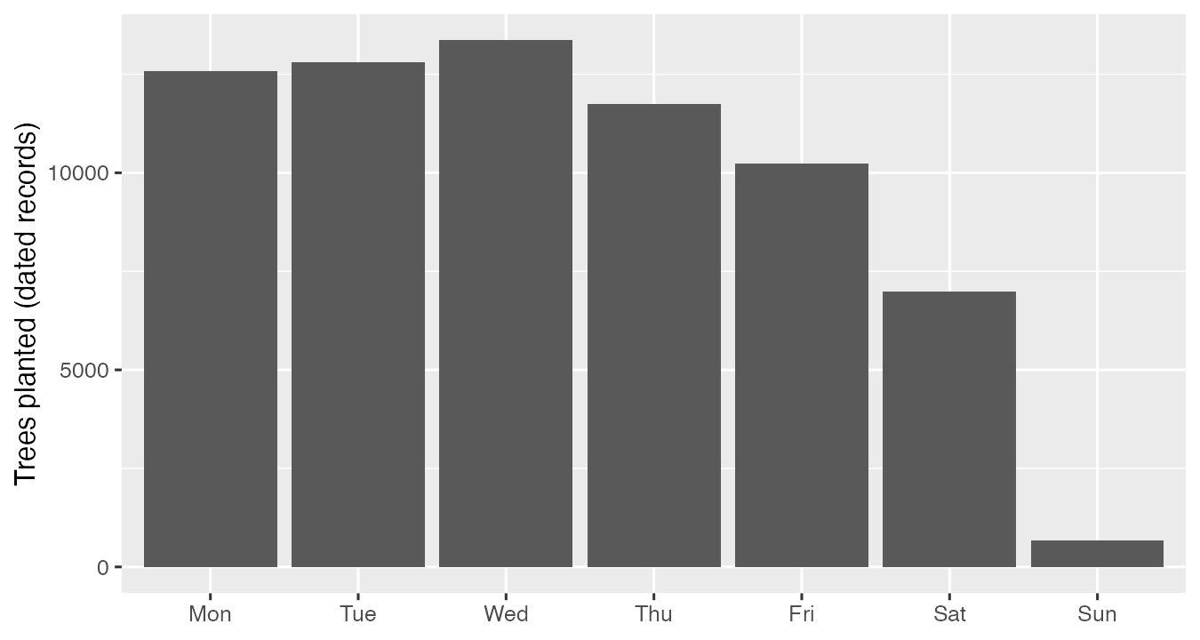
date read in as a Date, so there is nothing to parse. But 124,610 trees (65%) have no planting date, so any figure of plantings describes dated records only, and its caption has to say so.
planted <- trees |>
  filter(!is.na(date)) |>
  mutate(year = year(date),
         month = month(date, label = TRUE),
         weekday = wday(date, label = TRUE, week_start = 1))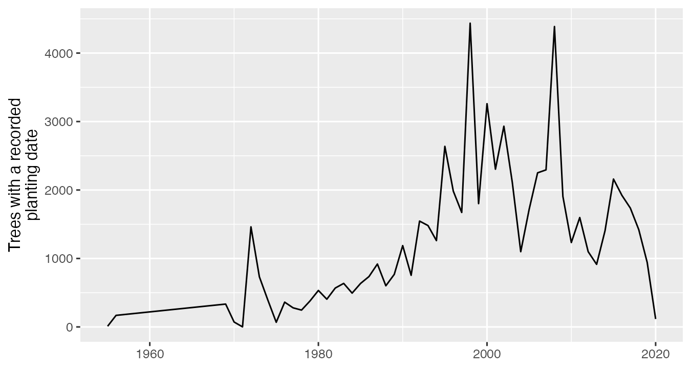
The file ends in January 2020, and recent plantings may not be entered yet, so the drop after 2016 is not evidence of fewer trees.
By day of the week, plantings follow the work week: Saturday is 10.2% of dated plantings and Sunday 1.0%. The dates record when crews and permit holders did the work. (Do not read caretaker as “who planted”: it is who maintains the tree now.)
12.5.5 Tables and inline values in your report
Your draft needs a small summary table and numbers in sentences. A gt table chunk in report.qmd:
#| label: tbl-top-trees
#| tbl-cap: "The five most common street trees in San Francisco."
trees_sp |>
  filter(!is.na(common)) |>
  count(common, sort = TRUE) |>
  head(5) |>
  gt() |>
  cols_label(common = "Common name", n = "Street trees") |>
  fmt_number(columns = n, decimals = 0)
The label must start with tbl- so Quarto numbers it as a table, the same way figure labels start with fig-. Refer to it in the text with @tbl-top-trees. If library(gt) fails, run install.packages("gt") once.
An inline value is R code inside a sentence. Type this in the text of report.qmd, not in a chunk:
The city lists `r format(nrow(trees), big.mark = ",")` street trees.It renders as “The city lists 192,987 street trees.” A number you type by hand goes stale the moment your data change; an inline value is recomputed every render. The object (trees here) must be created in a chunk above the sentence.
12.6 Common Problems
| You see | Why | Fix |
|---|---|---|
Expected 2 pieces in each element of species |
Some rows have no delimiter | Add too_few = "align_start" |
| Some rows did not split | Delimiter with spaces (" :: ") and rows without the trailing space |
Split on "::", then str_trim() |
"Tree(s)" or "" in your top-10 bar chart |
Placeholders are text, not NA |
na_if() each one after the split |
str_detect(x, "Width") finds 0 rows |
You lowercased first | Match the case you have: "width" |
Warnings about parsing failures from parse_number() inside if_else() |
if_else() computes both branches for every row |
Use str_extract() and as.numeric(), or ignore if only the other branch is affected |
An NA bar in a lumped bar chart |
fct_lump_n() before removing NA |
filter(!is.na(col)) first |
Bars still alphabetical after arrange() |
ggplot ignores row order | Order the factor: fct_infreq(), fct_reorder() |
| “Other” in the middle of the bars | Other outranks some named levels | fct_relevel(x, "Other", after = Inf) after fct_infreq() |
| Inline value shows the code, or an error on render | The object is created below the sentence, or backticks are missing | Create it in a chunk above; type a backtick, r, a space, the code, a backtick |
12.7 Try It
In your Module 05 repo, class/week_09_follow_along.R: Sections 1-4 with Challenges 1 and 2, then Section 5 in your own project report.qmd.
12.7.1 In-Class Challenge Hints
Try each step for a few minutes before opening a hint.
TipChallenge 1, Step 1, Hint 1: the plan
Start from trees_sp, where common is its own column. Remove the rows with no common name, count the names, keep the top five.
TipChallenge 1, Step 1, Hint 2: closer
trees_sp |> filter(!is.na(common)) |> count(common, sort = TRUE) |> head(5). London Plane (11,557) is first.
TipChallenge 1, Step 2, Hint 1: the plan
You want rows whose common name contains a word. Which stringr function returns TRUE or FALSE for that? Then count the rows.
TipChallenge 1, Step 2, Hint 2: closer
trees_sp |> filter(str_detect(common, "Cherry")) |> nrow() gives 14,571. It counts Cherry Plum, Kwanzan Flowering Cherry, and every other name with “Cherry” in it.
TipChallenge 2, Hint 1: the plan
caretaker needs no cleaning, so start from trees. Lump first, then order the levels inside aes().
TipChallenge 2, Hint 2: closer
trees |> mutate(caretaker = fct_lump_n(caretaker, n = 3)) |> ggplot(aes(y = fct_rev(fct_infreq(caretaker)))) + geom_bar(). Other (19 small groups together, 2,602 trees) outranks SFUSD (1,081), so it is third.
12.8 Connect To The Assignment
There is no Assignment 09. Assignment 08 (NOAA tornadoes) is due Sun Nov 22, 11:59 PM.
For your project draft (due Sun Nov 29): if your data have a text column with codes or mixed spellings, a category with many levels, or dates, this chapter is the pattern. Say each decision in your report (which placeholders became NA, what “Other” holds, which rows have dates). Add at least one summary table with a tbl- label and caption, and use inline values for the numbers in your sentences.